最短路径
最短路径应用的图是加权有向图
加权有向图的数据结构:
首先定义的是加权有向边的数据类型:1
2
3
4
5
6
7
8
9
10
11
12
13
14
15
16
17
18
19
20
21
22
23
24
25
26
27
28
29
30
31
32
33
34
35
36
37
38
39
40
41
42
43
44
45
46
47
48
49
50
51
52
53
54
55
56
57
58
59
60
61public class DirectEdge {
private int v;//边的起点
private int w;//边的终点
private double weight;//边的权重
public DirectEdge(int v,int w,double weight){
this.v=v;
this.w=w;
this.weight=weight;
}
public double weight(){
return weight;
}
public int from(){
return v;
}
public int to(){
return w;
}
public String toString(){
return String.format("%d->%d %.2f", v,w,weight);
}
} ```
在加权有向边的基础上定义加权有向图
```java
public class EdgeWeightDigraph {
private int V;
private int E;
private Bag<DirectEdge>[] adj;
public EdgeWeightDigraph(int V){
this.V=V;
this.E=0;
adj=(Bag<DirectEdge>[])new Bag[V];
for(int v=0;v<V;v++){
adj[v]=new Bag<DirectEdge>();
}
}
public int V(){
return V;
}
public int E(){
return E;
}
public void addEdge(DirectEdge e){
int v=e.from();
adj[v].add(e);
E++;
}
public Iterable<DirectEdge> adj(int v){
return adj[v];
}
public Iterable<DirectEdge> edges(){
Bag<DirectEdge> bag=new Bag<DirectEdge>();
for(int v=0;v<V;v++){
for(DirectEdge e:adj[v]){
bag.add(e);
}
}
return bag;
}
}
最短路径:从图的一个顶点到达另一个顶点的成本最小(权重和最小)的路径,这里的最短路径是单点最短路径
最短路径树: 给定一幅加权有向图和顶点s,可以找到一个以s为起点的最小路径树,他是图的一幅子图,包含了顶点s和所有s可达的顶点。树的根节点是s,树的每一条路径都是有向图中的一条最短路径
最短路径算法原理
边的松弛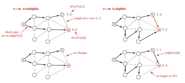
顶点的松弛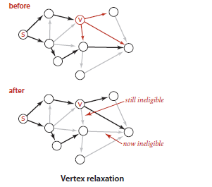
最短路径的最优条件:
一幅有向加权图G,顶点s为起点,distTo[]保存着起点s到任意顶点v的路径长度,若s到v不可达,该值为无穷大。当且仅当对于从v到w的任意一条边e,满足distTo[w]<=distTo[v]+e.weight()条件时,才是最短路径
Dijkstra算法
- 算法思想
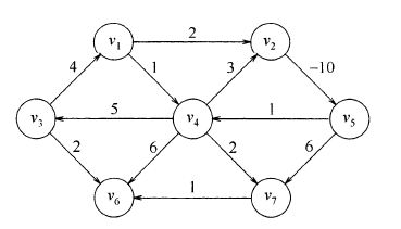
1) 首先Dijkstra算法只适用在权值非负的加权有向图
如下图所示,E(v2,v5)为负值,如果想找到v5到v4的最短路径,那么这一条路径:v5->v4->v2->v5->v4的权值之和为-6,如此一直沿着这条路径循环,那么v5到v4的路径权重之和会越来越小,趋近于负无穷,那么这两个顶点之间的最短路径无法确定。我们称图中这样的循环为负值圈,有向图中出现负值圈时,最短路径的问题就无法确定。
2)Dijkstra算法的思想
首先确定源点s,dist[v]表示的是从s到v的最短路径距离
Dijkstra算法每次从没有确定最短路径的顶点中选择dist[]值最小的顶点v,对v的所有边进行松弛,如此操作直到确定所有顶点的最短路径 算法实现
1
2
3
4
5
6
7
8
9
10
11
12
13
14
15
16
17
18
19
20
21
22
23
24
25
26
27
28
29
30
31
32
33
34
35
36
37
38
39
40
41
42
43
44
45
46
47
48
49
public class Dijkstra {
private DirectEdge[] edgeTo;
private double[] distTo;
private IndexMinPQ<Double> pq;
public Dijkstra(EdgeWeightDigraph G,int s){
edgeTo=new DirectEdge[G.V()];
distTo=new double[G.V()];
pq=new IndexMinPQ<Double>(G.V());
//初始化distTo所有项为正无穷
for(int v=0;v<G.V();v++){
distTo[v]=Double.POSITIVE_INFINITY;
}
//起始点设置为0
distTo[s]=0.0;
//将起始点入队
pq.insert(s, 0.0);
while(!pq.isEmpty()){
relax(G,pq.deleteMin());
}
}
private void relax(EdgeWeightDigraph G,int v){
for(DirectEdge e:G.adj(v)){
int w=e.to();
if(distTo[w]>distTo[v]+e.weight()){
distTo[w]=distTo[v]+e.weight();
edgeTo[w]=e;
if(pq.contains(w)){
pq.changeKey(w, distTo[w]);
}else{
pq.insert(w, distTo[w]);
}
}
}
}
public boolean hasPathTo(int v){
return distTo[v]<Double.POSITIVE_INFINITY;
}
public double distTo(int v){
return distTo[v];
}
public Iterable<DirectEdge> pathTo(int v){
Stack<DirectEdge> stack=new Stack<DirectEdge>();
while(edgeTo[v]!=null){
stack.push(edgeTo[v]);
v=edgeTo[v].from();
}
return stack;
}
}算法分析
Dijkstra算法时间复杂度取决于存储顶点的数据结构
上面算法的实现使用的是最小优先队列,每次删除最小距离顶点时间复杂度为logV,整个算法需要对每条边松弛,所以基于最小优先队列的Dijkstra算法的时间复杂度为ElogV
基于拓扑排序的最短路径算法
算法原理
将图按照拓扑排序的顺序放松顶点这种算法只能应用在无环有向图中,并且它允许图的边的权重是负值,他还能解决相关的问题比如最长路径
- 算法实现
1
2
3
4
5
6
7
8
9
10
11
12
13
14
15
16
17
18
19
20
21
22
23
24
25
26
27
28
29
30
31
32
33
34
35
36
37
38
39
40
//利用拓扑排序实现的最短路径算法
public class AcyclicSP {
private DirectEdge[] edgeTo;
private double[] distTo;
public AcyclicSP(EdgeWeightDigraph G,int s){
edgeTo=new DirectEdge[G.V()];
distTo=new double[G.V()];
for(int v=0;v<G.V();v++){
distTo[v]=Double.POSITIVE_INFINITY;
}
distTo[s]=0.0;
TopoEdgeWeight top=new TopoEdgeWeight(G);
for(int v:top.order()){
relax(G,v);
}
}
private void relax(EdgeWeightDigraph G,int v){
for(DirectEdge e:G.adj(v)){
int w=e.to();
if(distTo[w]>distTo[v]+e.weight()){
distTo[w]=distTo[v]+e.weight();
edgeTo[w]=e;
}
}
}
public boolean hasPathTo(int v){
return distTo[v]<Double.POSITIVE_INFINITY;
}
public double distTo(int v){
return distTo[v];
}
public Iterable<DirectEdge> pathTo(int v){
Stack<DirectEdge> stack=new Stack<DirectEdge>();
while(edgeTo[v]!=null){
stack.push(edgeTo[v]);
v=edgeTo[v].from();
}
return stack;
}
}
在查找最短路径之前需要对图进行拓扑排序1
2
3
4
5
6
7
8
9
10
11
12
13
14
15
16
17
18
19
20
21
22
23
24
25
26
27
28
29
30
31
32
33
34
35
36
37
38
39
40
41
42
43
44
45
46
47
48
49
50
51
52
53
54
55
56
57
58
59
60
61
62
63
64
65
66
67
68
69
70
71
72
73
74
75
76
77
78public class TopoEdgeWeight {
private boolean marked[];
private Stack<Integer> stack;
public TopoEdgeWeight(EdgeWeightDigraph G){
marked=new boolean[G.V()];
stack=new Stack<Integer>();
EdgeWeightDigraphCycle cycle=new EdgeWeightDigraphCycle(G);
if(!cycle.hasCycle()){
TopoSort(G);
}
}
private void TopoSort(EdgeWeightDigraph G){
for(int v=0;v<G.V();v++){
if(!marked[v]){
dfs(G,v);
}
}
}
private void dfs(EdgeWeightDigraph G,int v){
marked[v]=true;
for(DirectEdge e:G.adj(v)){
if(!marked[e.to()]){
dfs(G,e.to());
}
}
stack.push(v);
}
public Iterable<Integer> order(){
return stack;
}
}```
在拓扑排序之前需要检查图是不是无环图
```java
public class EdgeWeightDigraphCycle {
private boolean[] marked;
private DirectEdge[] edgeTo;
private Stack<DirectEdge> cycle;
private boolean[] onStack;
public EdgeWeightDigraphCycle(EdgeWeightDigraph G){
marked=new boolean[G.V()];
edgeTo=new DirectEdge[G.V()];
onStack=new boolean[G.V()];
for(int v=0;v<G.V();v++){
if(!marked[v]){
dfs(G,v);
}
}
}
private void dfs(EdgeWeightDigraph G,int v){
marked[v]=true;
onStack[v]=true;
for(DirectEdge e:G.adj(v)){
int w=e.to();
if(hasCycle()){
return;
}else if(!marked[w]){
edgeTo[w]=e;
dfs(G,w);
}else if(onStack[w]){
cycle=new Stack<DirectEdge>();
DirectEdge f=e;
while(f.from()!=w){
cycle.push(f);
f=edgeTo[f.from()];
}
cycle.push(f);
return;
}
}
onStack[v]=false;
}
public boolean hasCycle(){
return cycle!=null;
}
public Iterable<DirectEdge> cycle(){
return cycle;
}
}
- 算法分析
基于拓扑排序的最短路径算法是一种比Dijkstra算法更快更简单的在无环加权有向图中找到最短路径的算法
基于拓扑排序的最短路径算法的时间复杂度是O(V+E)
Floyd算法
算法原理
从任意节点v到节点w最短路径有两种情况:第一种是直接从v到w;第二种是从v经过若干个节点到达w,对图中的每个节点k,检查dist(v,k)+dist(k,w)<dist(v,w)是否成立,如果成立,那么更新v到w的最短路径为dist(v,k)+dist(k,w),如此当我们遍历完图中所有的节点之后,v到w的最短路径和最短距离就确定了。此算法就是一任意的顺序放松图中所有的边,重复V轮。算法实现
三重循环实现for (int k=0; k<n; ++k) { for (int i=0; i<n; ++i) { for (int j=0; j<n; ++j) { if (dist[i][k] + dist[k][j] < dist[i][j] ) { dist[i][j] = dist[i][k] + dist[k][j]; path[i][j] = path[k][j]; } } } }算法分析
Floyd算法的时间复杂度为:O(V3)
Bellman-Ford算法
Bellman-ford算法是求含负权图的单源最短路径算法,效率很低,但代码很容易写
- 算法原理
利用队列 - 算法实现
public class BellmanFord { private double[] distTo; private DirectEdge[] edgeTo; private boolean[] onQ;//该顶点是否在队列中 private Queue<Integer> queue;//用于存放将被放松的顶点 private int cont;//放松的次数 private Iterable<DirectEdge> cycle; public BellmanFord(EdgeWeightDigraph G,int s){ distTo=new double[G.V()]; edgeTo=new DirectEdge[G.V()]; onQ=new boolean[G.V()]; queue=new Queue<Integer>(); for(int v=0;v<G.V();v++){ distTo[v]=Double.POSITIVE_INFINITY; } queue.enqueue(s); onQ[s]=true; distTo[s]=0.0; while(!queue.isEmpty() && hasNegativeCycle()){ int v=queue.dequeue(); onQ[v]=false; relax(G,v); } } private void relax(EdgeWeightDigraph G,int v){ for(DirectEdge e:G.adj(v)){ int w=e.to(); if(distTo[w]>distTo[v]+e.weight()){ distTo[w]=distTo[v]+e.weight(); edgeTo[w]=e; if(!onQ[w]){ queue.enqueue(w); onQ[w]=true; } } if(cont++ % G.V() ==0){ findNegativeCycle(); } } } public void findNegativeCycle(){ int V=edgeTo.length; EdgeWeightDigraph bf=new EdgeWeightDigraph(V); for(int v=0;v<V;v++){ if(edgeTo[v]!=null){ bf.addEdge(edgeTo[v]); } } EdgeWeightDigraphCycle cf=new EdgeWeightDigraphCycle(bf); cycle=cf.cycle(); } public boolean hasNegativeCycle(){ return cycle!=null; } public Iterable<DirectEdge> negativeCycle(){ return cycle; } public boolean hasPathTo(int v){ return distTo[v]<Double.POSITIVE_INFINITY; } public double distTo(int v){ return distTo[v]; } public Iterable<DirectEdge> pathTo(int v){ Stack<DirectEdge> stack=new Stack<DirectEdge>(); while(edgeTo[v]!=null){ stack.push(edgeTo[v]); v=edgeTo[v].from(); } return stack; } } - 算法分析
BellmanFord算法的时间复杂度一般情况为O(E+V),最坏情况为O(VE)